Note

This page was generated from docs/source/notebooks/user_prior.ipynb. An interactive version of this notebook can be run using Binder by clicking

Note that if you wish to run this notebook on your own, you’ll need to have matplotlib and seaborn installed.

User-defined prior distribution

from pyunfold import iterative_unfold
from pyunfold.callbacks import Logger

import numpy as np
np.random.seed(2)
import matplotlib.pyplot as plt
import seaborn as sns

%matplotlib inline

sns.set_context(context='poster')
plt.rcParams['figure.figsize'] = (10, 8)
plt.rcParams['lines.markeredgewidth'] = 2

Example dataset

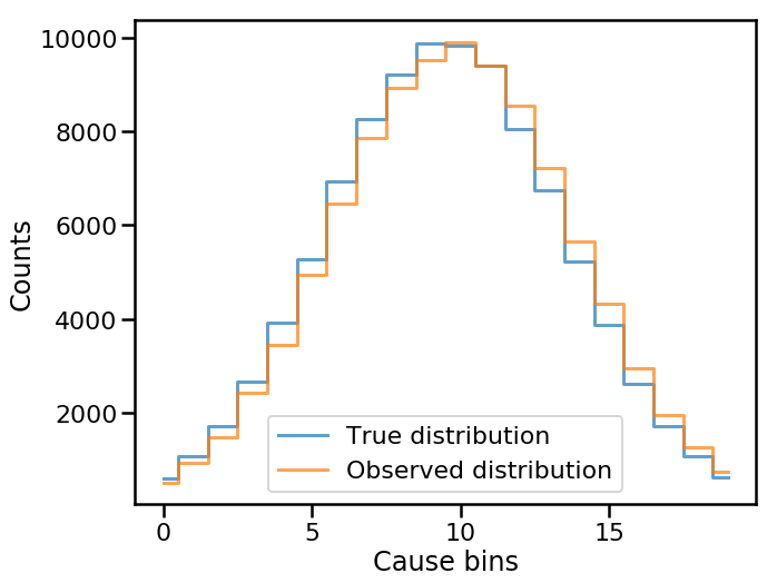
We’ll generate the same example dataset that is used in the Getting Started tutorial, i.e. a Gaussian sample that is smeared by some noise.

# True distribution
num_samples = int(1e5)
true_samples = np.random.normal(loc=10.0, scale=4.0, size=num_samples)
bins = np.linspace(0, 20, 21)
num_causes = len(bins) - 1
data_true, _ = np.histogram(true_samples, bins=bins)

# Observed distribution
random_noise = np.random.normal(loc=0.3, scale=0.5, size=num_samples)
observed_samples = true_samples + random_noise
data_observed, _ = np.histogram(observed_samples, bins=bins)
data_observed_err = np.sqrt(data_observed)

# Efficiencies
efficiencies = np.ones_like(data_observed, dtype=float)
efficiencies_err = np.full_like(efficiencies, 0.1, dtype=float)

# Response matrix
response_hist, _, _ = np.histogram2d(observed_samples, true_samples, bins=bins)
response_hist_err = np.sqrt(response_hist)

# Normalized response
column_sums = response_hist.sum(axis=0)
normalization_factor = efficiencies / column_sums

response = response_hist * normalization_factor
response_err = response_hist_err * normalization_factor

We can see what the true and observed distributions look like for this example dataset

fig, ax = plt.subplots(figsize=(10, 8))
ax.step(np.arange(len(data_true)), data_true, where='mid', lw=3,
        alpha=0.7, label='True distribution')
ax.step(np.arange(len(data_observed)), data_observed, where='mid', lw=3,
        alpha=0.7, label='Observed distribution')
ax.set(xlabel='Cause bins', ylabel='Counts')
ax.legend()
plt.show()

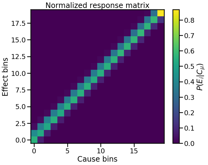
as well as the normalized response matrix

fig, ax = plt.subplots(figsize=(10, 8))
im = ax.imshow(response, origin='lower')
cbar = plt.colorbar(im, label='$P(E_i|C_{\mu})$')
ax.set(xlabel='Cause bins', ylabel='Effect bins',
       title='Normalized response matrix')
plt.show()

Custom Priors

The default initial prior used in PyUnfold is the uniform prior (i.e. each cause bin is given an equal weighting). We can test other priors by providing a normalized distribution via the prior parameter in the iterative_unfold function.

Several convenience functions for calculating commonly used prior distributions exist in the pyunfold.priors module. However, any normalized array-like object (i.e. the items sum to 1) can be passed to prior and used as the initial prior in an unfolding.

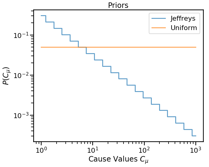
One commonly used prior is the non-informative Jeffreys’ prior. The analytic form of this prior is given by

\[P(C_{\mu})^{\text{Jeffreys}} = \frac{1}{\log \left( C_{\text{max}} / C_{\text{min}}\right) \, C_{\mu}}\]

where \(C_{\text{max}}\) and \(C_{\text{min}}\) are the maximum and minimum possible cause values, and \(C_{\mu}\) is the value of the \(\mu\)th cause bin. Here we’ll assume that the cause range covers three orders of magnitude, that is \(C_{\mu} \in [1, 10^3]\).

from pyunfold.priors import jeffreys_prior, uniform_prior

# Cause limits
cause_lim = np.logspace(0, 3, num_causes)

# Uniform and Jeffreys' priors
uni_prior = uniform_prior(num_causes)
jeff_prior = jeffreys_prior(cause_lim)

The uniform_prior and jeffreys_prior functions calculate their corresponding prior distributions and return NumPy ndarrays containing these distributions. For more information about these functions, see the priors API documentation.

print(type(uni_prior))
print('uni_prior = {}'.format(uni_prior))

<class 'numpy.ndarray'>
uni_prior = [0.05 0.05 0.05 0.05 0.05 0.05 0.05 0.05 0.05 0.05 0.05 0.05 0.05 0.05
 0.05 0.05 0.05 0.05 0.05 0.05]

print(type(jeff_prior))
print('jeff_prior = {}'.format(jeff_prior))

<class 'numpy.ndarray'>
jeff_prior = [3.05019251e-01 2.12047186e-01 1.47413676e-01 1.02480926e-01
 7.12440013e-02 4.95283165e-02 3.44317288e-02 2.39366898e-02
 1.66406143e-02 1.15684352e-02 8.04229282e-03 5.59094404e-03
 3.88678402e-03 2.70206425e-03 1.87845560e-03 1.30588880e-03
 9.07844487e-04 6.31126948e-04 4.38754908e-04 3.05019251e-04]

fig, ax = plt.subplots(figsize=(10, 8))
ax.step(cause_lim, jeff_prior, where='mid', lw=3,
        alpha=0.7, label='Jeffreys')
ax.step(cause_lim, uni_prior, where='mid', lw=3,
        alpha=0.7, label='Uniform')
ax.set(xlabel='Cause Values $C_{\mu}$', ylabel='$P(C_{\mu})$',
       title='Priors')
plt.xscale('log')
plt.yscale('log')
plt.legend()
plt.show()

Unfolding

Now we can run the unfolding with the Jeffreys’ prior and compare to the default uniform prior as well as the true cause distribution.

print('Running with uniform prior...')
unfolded_uniform = iterative_unfold(data=data_observed,
                                    data_err=data_observed_err,
                                    response=response,
                                    response_err=response_err,
                                    efficiencies=efficiencies,
                                    efficiencies_err=efficiencies_err,
                                    ts='ks',
                                    ts_stopping=0.01,
                                    callbacks=[Logger()])

print('\nRunning with Jeffreys prior...')
unfolded_jeffreys = iterative_unfold(data=data_observed,
                                     data_err=data_observed_err,
                                     response=response,
                                     response_err=response_err,
                                     efficiencies=efficiencies,
                                     efficiencies_err=efficiencies_err,
                                     prior=jeff_prior,
                                     ts='ks',
                                     ts_stopping=0.01,
                                     callbacks=[Logger()])

Running with uniform prior...
Iteration 1: ts = 0.1460, ts_stopping = 0.01
Iteration 2: ts = 0.0060, ts_stopping = 0.01

Running with Jeffreys prior...
Iteration 1: ts = 0.7231, ts_stopping = 0.01
Iteration 2: ts = 0.0171, ts_stopping = 0.01
Iteration 3: ts = 0.0006, ts_stopping = 0.01

bin_midpoints = (bins[1:] + bins[:-1]) / 2
fig, ax = plt.subplots(figsize=(10, 8))
ax.hist(true_samples, bins=bins, histtype='step', lw=3,
        alpha=0.7,
        label='True distribution')

ax.errorbar(bin_midpoints, unfolded_uniform['unfolded'],
            yerr=unfolded_uniform['sys_err'],
            alpha=0.7,
            elinewidth=3,
            capsize=4,
            ls='None', marker='.', ms=10,
            label='Unfolded - Uniform Prior')

ax.errorbar(bin_midpoints, unfolded_jeffreys['unfolded'],
            yerr=unfolded_jeffreys['sys_err'],
            alpha=0.7,
            elinewidth=3,
            capsize=4,
            ls='None', marker='.', ms=10,
            label='Unfolded - Jeffreys Prior')

ax.set(xlabel='Cause bins', ylabel='Counts')
plt.legend()
plt.show()

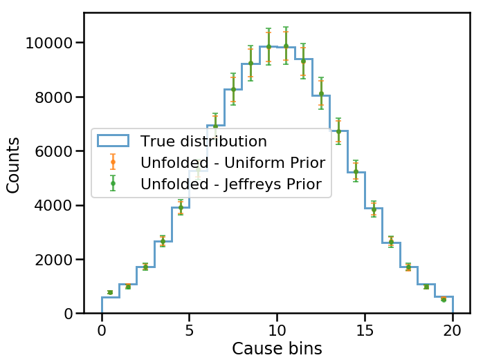
The unfolded distributions are consistent with each other as well as with the true distribution! Thus, our results are robust with respect to these two smooth initial priors.

For information about how un-smooth priors can affect an unfolding see the smoothing via spline regularization example.