Note

This page was generated from docs/source/notebooks/multivariate.ipynb. An interactive version of this notebook can be run using Binder by clicking

Note that if you wish to run this notebook on your own, you’ll need to have matplotlib and seaborn installed.

Multivariate unfolding

from pyunfold import iterative_unfold
from pyunfold.callbacks import Logger

import numpy as np
np.random.seed(2)
import matplotlib.pyplot as plt
import seaborn as sns

%matplotlib inline

sns.set_context(context='poster')
plt.rcParams['figure.figsize'] = (10, 8)
plt.rcParams['lines.markeredgewidth'] = 2

Example dataset

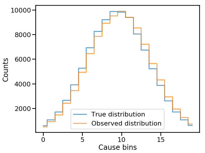
We’ll generate the same example dataset that is used in the Getting Started tutorial, i.e. a Gaussian sample that is smeared by some noise.

# True distribution
num_samples = int(1e5)
true_samples = np.random.normal(loc=10.0, scale=4.0, size=num_samples)
bins = np.linspace(0, 20, 21)
num_causes = len(bins) - 1
data_true, _ = np.histogram(true_samples, bins=bins)

# Observed distribution
random_noise = np.random.normal(loc=0.3, scale=0.5, size=num_samples)
observed_samples = true_samples + random_noise
data_observed, _ = np.histogram(observed_samples, bins=bins)
data_observed_err = np.sqrt(data_observed)

# Efficiencies
efficiencies = np.ones_like(data_observed, dtype=float)
efficiencies_err = np.full_like(efficiencies, 0.1, dtype=float)

# Response matrix
response_hist, _, _ = np.histogram2d(observed_samples, true_samples, bins=bins)
response_hist_err = np.sqrt(response_hist)

# Normalized response
column_sums = response_hist.sum(axis=0)
normalization_factor = efficiencies / column_sums

response = response_hist * normalization_factor
response_err = response_hist_err * normalization_factor

We can see what the true and observed distributions look like for this example dataset

fig, ax = plt.subplots()
ax.step(np.arange(len(data_true)), data_true, where='mid', lw=3,
        alpha=0.7, label='True distribution')
ax.step(np.arange(len(data_observed)), data_observed, where='mid', lw=3,
        alpha=0.7, label='Observed distribution')
ax.set(xlabel='Cause bins', ylabel='Counts')
ax.legend()
plt.show()

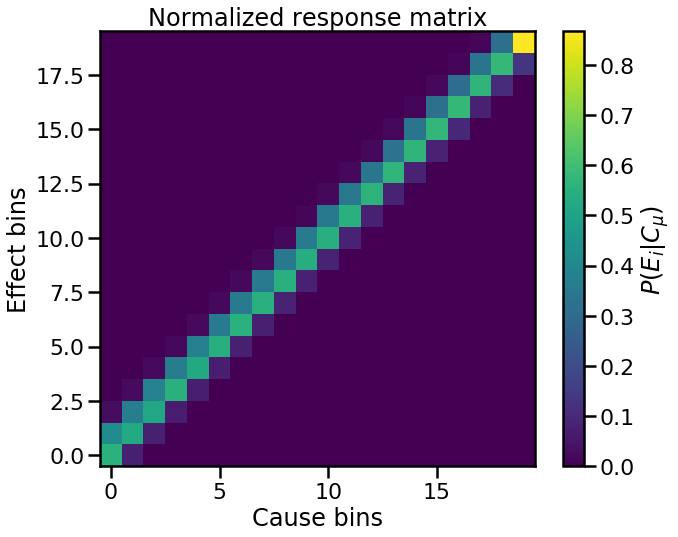
as well as the normalized response matrix

fig, ax = plt.subplots()
im = ax.imshow(response, origin='lower')
cbar = plt.colorbar(im, label='$P(E_i|C_{\mu})$')
ax.set(xlabel='Cause bins', ylabel='Effect bins',
       title='Normalized response matrix')
plt.show()

Cause Groups

To illustrate the generalization to multivariate unfolding, we consider a set of effects originating from two different cause types having their own ranges. We can assign a new superscript \(i\) to denote these types:

\[C_{\mu}^{i} \text{ where } i \in [1,2]\]

and the subscript \(\mu\) runs over the respective number of causes in each type \(\, n_{C1}\) and \(\, n_{C2}\).

But since the PyUnfold doesn’t care how we label the bins, we can simply redefine our cause index \(\mu\) to run over a larger index range. Hence,

\[C_{\mu}^i \rightarrow C_{\mu} \text{ where } \mu \in [1, \, n_{C1} + n_{C2}]\]

Thus, given a general multidimensional (\(i>1\)) response matrix, we can effectively unroll it onto a two dimensional array and still use PyUnfold.

Example—two identical cause groups

Here we use two identical cause groups, simply copying our original response matrix along the cause axis.

# Response with two groups
response_hist_groups = np.concatenate((response_hist, response_hist), axis=1)
response_hist_groups_err = np.sqrt(response_hist_groups)

# Efficiencies with two groups
efficiencies_groups = np.ones(response_hist_groups.shape[1], dtype=float)
efficiencies_groups_err = np.full_like(efficiencies_groups, 0.1, dtype=float)
num_causes = response_hist_groups.shape[1]

# Scale by efficiency
column_sums_groups = response_hist_groups.sum(axis=0)
normalization_factor_groups = efficiencies_groups / column_sums_groups

# Response matrix with two groups
response_groups = response_hist_groups * normalization_factor_groups
response_groups_err = response_hist_groups_err * normalization_factor_groups

fig, ax = plt.subplots(figsize=(16, 8))
im = ax.imshow(response_groups, origin='lower')
plt.colorbar(im, label='$P(E_i|C_{\mu})$')
ax.set(xlabel='Cause bins', ylabel='Effect bins',
       title='Normalized response matrix - 2 groups')
plt.show()

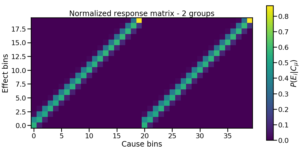
Now the two (identical) cause groups are unrolled clearly along the abscissa. Since the unfolding method is cause agnostic, we can perform an unfolding, remembering that we’ve kept the same observed data.

unfolded_results_groups = iterative_unfold(data=data_observed,
                                           data_err=data_observed_err,
                                           response=response_groups,
                                           response_err=response_groups_err,
                                           efficiencies=efficiencies_groups,
                                           efficiencies_err=efficiencies_groups_err,
                                           ts='ks',
                                           ts_stopping=0.01,
                                           callbacks=[Logger()])

Iteration 1: ts = 0.0730, ts_stopping = 0.01
Iteration 2: ts = 0.0030, ts_stopping = 0.01

fig, ax = plt.subplots()
ax.errorbar(np.arange(num_causes), unfolded_results_groups['unfolded'],
            yerr=unfolded_results_groups['sys_err'],
            alpha=0.7,
            elinewidth=3,
            capsize=4,
            ls='None', marker='.', ms=10)
ax.set(xlabel='Cause bins', ylabel='Counts',
        title='Group Unfolding')
plt.show()

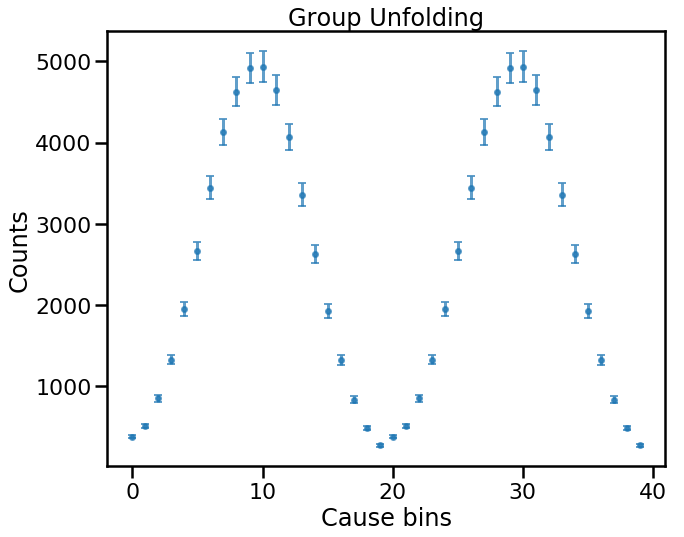
So the result is two equal copies of the causes. This makes sense because in our example we have simply considered two identical groups of causes, so they should contribute identically to producing the measured effects.

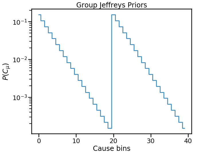
User Priors with Groups

What if we want to use the a user-defined prior (e.g. Jeffreys’ prior)? In this case, we have to setup the prior input to contain the priors we want for each group.

from pyunfold.priors import jeffreys_prior

# Cause limits
cause_lim = np.logspace(0, 3, num_causes // 2)

# Setup group Jeffreys' prior
prior_jeff_groups = np.concatenate([jeffreys_prior(cause_lim), jeffreys_prior(cause_lim)])
prior_jeff_groups = prior_jeff_groups / prior_jeff_groups.sum()

fig, ax = plt.subplots()
ax.step(np.arange(num_causes), prior_jeff_groups, where='mid', lw=3,
        alpha=0.8)
ax.set(xlabel='Cause bins', ylabel='$P(C_{\mu})$',
       title='Group Jeffreys Priors')
ax.set_yscale('log')
plt.show()

unfolded_results_groups_jeff = iterative_unfold(data=data_observed,
                                                data_err=data_observed_err,
                                                response=response_groups,
                                                response_err=response_groups_err,
                                                efficiencies=efficiencies_groups,
                                                efficiencies_err=efficiencies_groups_err,
                                                prior=prior_jeff_groups,
                                                ts='ks',
                                                ts_stopping=0.01,
                                                callbacks=[Logger()])

Iteration 1: ts = 0.3615, ts_stopping = 0.01
Iteration 2: ts = 0.0085, ts_stopping = 0.01

fig, ax = plt.subplots()
plt.errorbar(np.arange(num_causes), unfolded_results_groups_jeff['unfolded'],
             yerr=unfolded_results_groups_jeff['sys_err'],
             alpha=0.7,
             elinewidth=3,
             capsize=4,
             ls='None', marker='.', ms=10)

ax.set(xlabel='Cause bins', ylabel='Counts',
       title='Group Unfolding - Jeffreys Prior')
plt.show()
plt.show()

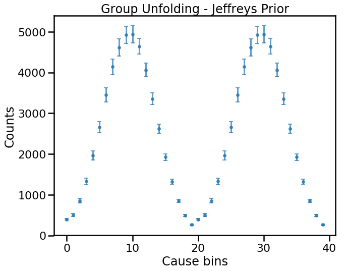
Again, we recover two copies of the causes.

Regularization with Groups

In general, groups of causes do not share continuity of the cause axis. In the above examples, the cause arrays are stacked next to each other, so while the unfolding method doesn’t care about the cause definitions, the default regularization smooths over all cause bins without regard to types.

PyUnfold implements group regularization, where smoothing of the unfolded distributions is performed only within designated cause types (i.e. each cause type is regularized independently). This is done by providing the SplineRegularizer function a groups list, defining a group identification for each cause bin.

from pyunfold.callbacks import SplineRegularizer

# Here we know we have two copies of the causes
n_c1 = response_groups.shape[1] // 2
n_c2 = response_groups.shape[1] // 2

groups = [0]*n_c1 + [1]*n_c2
print("Group definitions: \n{}".format(groups))

Group definitions:
[0, 0, 0, 0, 0, 0, 0, 0, 0, 0, 0, 0, 0, 0, 0, 0, 0, 0, 0, 0, 1, 1, 1, 1, 1, 1, 1, 1, 1, 1, 1, 1, 1, 1, 1, 1, 1, 1, 1, 1]

group_reg = SplineRegularizer(degree=3, smooth=1.25, groups=groups)

unfolded_results_groups_reg = iterative_unfold(data=data_observed,
                                               data_err=data_observed_err,
                                               response=response_groups,
                                               response_err=response_groups_err,
                                               efficiencies=efficiencies_groups,
                                               efficiencies_err=efficiencies_groups_err,
                                               ts='ks',
                                               ts_stopping=0.01,
                                               callbacks=[Logger(), group_reg])

Iteration 1: ts = 0.0730, ts_stopping = 0.01
Iteration 2: ts = 0.0030, ts_stopping = 0.01

fig, ax = plt.subplots()
ax.errorbar(np.arange(num_causes), unfolded_results_groups_reg['unfolded'],
            yerr=unfolded_results_groups_reg['sys_err'],
            alpha=0.7,
            elinewidth=3,
            capsize=4,
            ls='None', marker='.', ms=10)

ax.set(xlabel='Cause bins', ylabel='Counts',
       title='Group Unfolding - regularized')
plt.show()

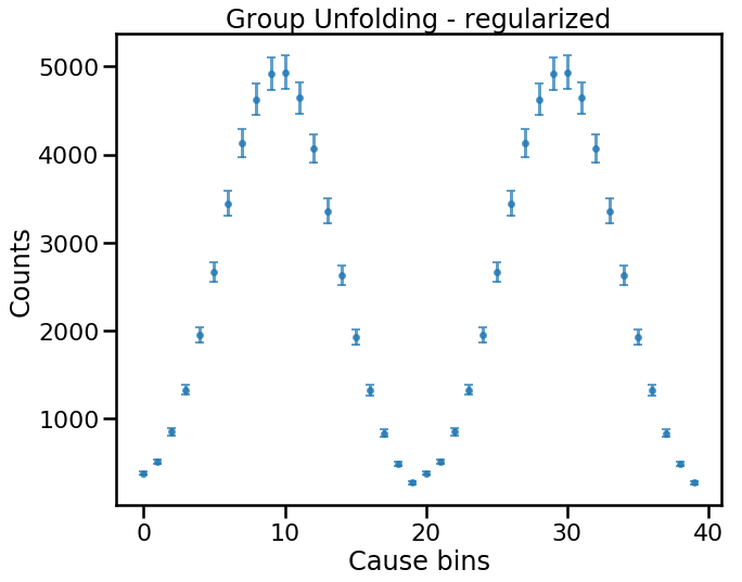
Again, for this simple example, everything looks fine.

However, if we consider a more complicated example, we’ll see the power of these implementations.

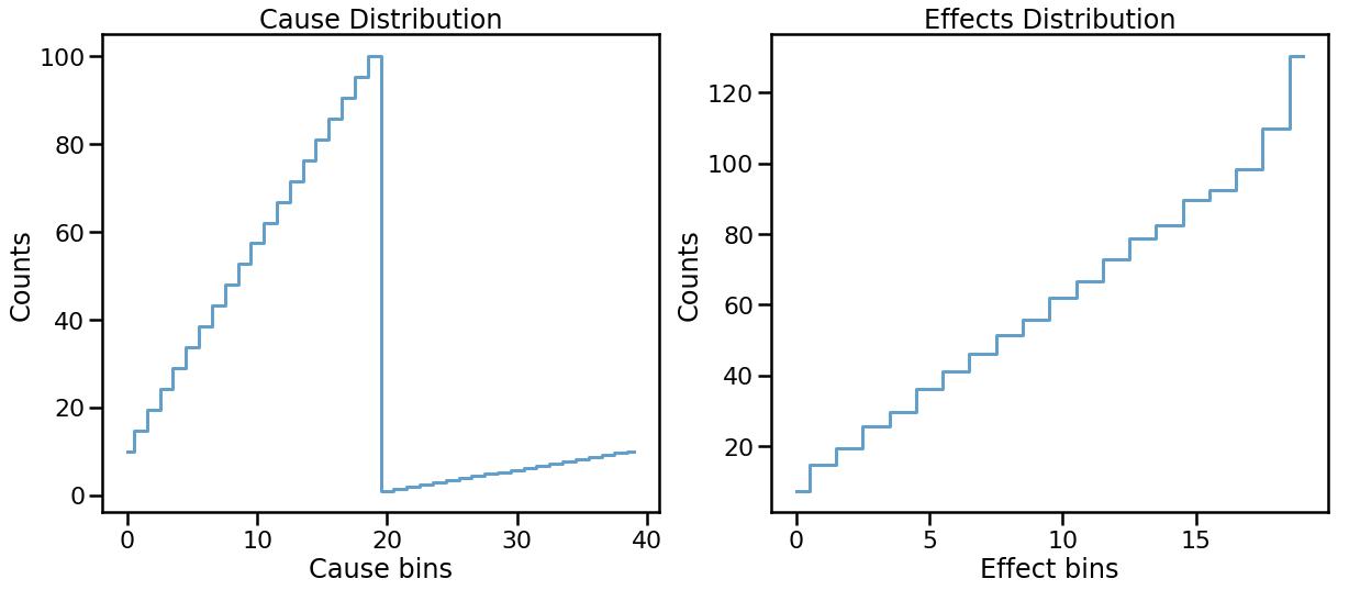
Pitfalls of multivariate unfolding

Let’s generate some more example data by keeping our two-type response matrix.

# True distribution
group_data_true = np.concatenate((np.linspace(10, 100, n_c1), np.linspace(1, 10, n_c2)))

# Observed data, no smearing
group_data_observed = response_groups.dot(group_data_true)
group_data_observed_err = np.sqrt(group_data_observed)

fig, (ax_1, ax_2) = plt.subplots(ncols=2, figsize=(20, 8))
# Cause distribution
ax_1.step(np.arange(num_causes), group_data_true, where='mid', lw=3,
         alpha=0.7, label='True distribution')
ax_1.set(xlabel='Cause bins', ylabel='Counts',
         title='Cause Distribution')

# Effects distribution
ax_2.step(np.arange(len(group_data_observed)), group_data_observed, where='mid', lw=3,
          alpha=0.7, label='Observed distribution')
ax_2.set(xlabel='Effect bins', ylabel='Counts',
         title='Effects Distribution')

plt.show()

# Setup all cause spline
spline_reg = SplineRegularizer(degree=3, smooth=5e6)

# Setup group spline
group_reg = SplineRegularizer(degree=3, smooth=1.25, groups=groups)

unfolded_results_groups_default_reg = iterative_unfold(data=group_data_observed,
                                                       data_err=group_data_observed_err,
                                                       response=response_groups,
                                                       response_err=response_groups_err,
                                                       efficiencies=efficiencies_groups,
                                                       efficiencies_err=efficiencies_groups_err,
                                                       ts='ks',
                                                       ts_stopping=0.01,
                                                       callbacks=[Logger(), spline_reg])

Iteration 1: ts = 0.0919, ts_stopping = 0.01
Iteration 2: ts = 0.0479, ts_stopping = 0.01
Iteration 3: ts = 0.0246, ts_stopping = 0.01
Iteration 4: ts = 0.0125, ts_stopping = 0.01
Iteration 5: ts = 0.0064, ts_stopping = 0.01

unfolded_results_groups_group_reg = iterative_unfold(data=group_data_observed,
                                                     data_err=group_data_observed_err,
                                                     response=response_groups,
                                                     response_err=response_groups_err,
                                                     efficiencies=efficiencies_groups,
                                                     efficiencies_err=efficiencies_groups_err,
                                                     ts='ks',
                                                     ts_stopping=0.01,
                                                     callbacks=[Logger(), group_reg])

Iteration 1: ts = 0.1070, ts_stopping = 0.01
Iteration 2: ts = 0.0011, ts_stopping = 0.01

fig, ax = plt.subplots()
ax.step(np.arange(num_causes), group_data_true, where='mid', lw=3,
        alpha=0.7, label='True Distribution')

ax.errorbar(np.arange(num_causes), unfolded_results_groups_group_reg['unfolded'],
            yerr=unfolded_results_groups_group_reg['sys_err'],
            alpha=0.7,
            elinewidth=3,
            capsize=4,
            ls='None', marker='.', ms=10,
            label='Group Regularization')

ax.errorbar(np.arange(num_causes), unfolded_results_groups_default_reg['unfolded'],
            yerr=unfolded_results_groups_default_reg['sys_err'],
            alpha=0.7,
            elinewidth=3,
            capsize=4,
            ls='None', marker='.', ms=10,
            label='Default Regularization')

ax.set(xlabel='Cause bins', ylabel='Counts',
       title='Group Unfolding')
ax.legend()
plt.show()

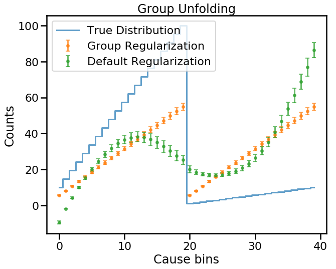
So, what’s going on here? There are actually two problems here.

1. It’s clear that the default regularization tries to connect the two cause groups in a smooth manner.
2. And while the group regularization is doing its best to smooth each group individually, it’s clear we are getting copies again. This is due to the prior assumption that all causes have equal probabilities.

Let’s redo this by giving a strong preference in the prior to one of the groups.

# Flat prior to each group, but one has stronger preference.
flat_pref_prior = np.concatenate((8.*np.ones(n_c1), np.ones(n_c1)))
flat_pref_prior = flat_pref_prior / flat_pref_prior.sum()

unfolded_results_groups_group_reg_prior = iterative_unfold(data=group_data_observed,
                                                           data_err=group_data_observed_err,
                                                           response=response_groups,
                                                           response_err=response_groups_err,
                                                           efficiencies=efficiencies_groups,
                                                           efficiencies_err=efficiencies_groups_err,
                                                           prior=flat_pref_prior,
                                                           ts='ks',
                                                           ts_stopping=0.01,
                                                           callbacks=[Logger(), group_reg])

Iteration 1: ts = 0.1900, ts_stopping = 0.01
Iteration 2: ts = 0.0018, ts_stopping = 0.01

fig, ax = plt.subplots()
ax.step(np.arange(num_causes), group_data_true, where='mid', lw=3,
        alpha=0.7, label='True Distribution')

ax.errorbar(np.arange(num_causes), unfolded_results_groups_group_reg_prior['unfolded'],
            yerr=unfolded_results_groups_group_reg_prior['sys_err'],
            alpha=0.7,
            elinewidth=3,
            capsize=4,
            ls='None', marker='.', ms=10,
            label='Group Regularization')

ax.set(xlabel='Cause bins', ylabel='Counts',
       title='Group Unfolding')
ax.legend()
plt.show()

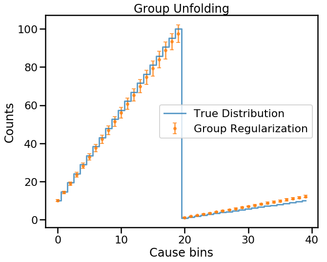
Now we’re starting to get something that looks right.

However, we are still using two identical copies of the response matrix which means that we’re considering the same sets of causes, just split up into two groups.

This also demonstrates another potential issue with doing group unfolding: if there is high degree of degeneracy between the respective response functions, then the unfolding results will be strongly dependent on intial priors.

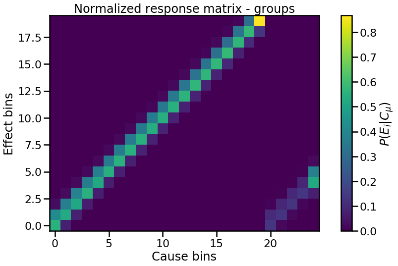
The solution to this is to ensure that the cause group response matrices have different structure, for example by having different normalizations (efficiency). We demonstrate this below to finish.

# Response with two groups having different structures
n_c1 = len(response_hist)
n_c2 = 5
response_hist_groups = np.concatenate((response_hist, response_hist[:,0:n_c2]), axis=1)
response_hist_groups_err = np.sqrt(response_hist_groups)

# Efficiencies with two groups
efficiencies_groups = np.ones(response_hist_groups.shape[1], dtype=float)
efficiencies_groups_err = np.full_like(efficiencies_groups, 0.1, dtype=float)
# Make the second group 25% efficient
efficiencies_groups[0:n_c1] *= 1
efficiencies_groups[n_c1:-1] *= 0.25
efficiencies_groups_err = np.full_like(efficiencies_groups, 0.1, dtype=float)

# Scale by efficiency
column_sums_groups = response_hist_groups.sum(axis=0)
normalization_factor_groups = efficiencies_groups / column_sums_groups

# Response matrix with two groups
response_groups = response_hist_groups * normalization_factor_groups
response_groups_err = response_hist_groups_err * normalization_factor_groups

groups = [0]*n_c1 + [1]*n_c2
print("Group definitions: {}".format(groups))

Group definitions: [0, 0, 0, 0, 0, 0, 0, 0, 0, 0, 0, 0, 0, 0, 0, 0, 0, 0, 0, 0, 1, 1, 1, 1, 1]

group_reg = SplineRegularizer(degree=3, smooth=1.25, groups=groups)

fig, ax = plt.subplots(figsize=(16, 8))
im = ax.imshow(response_groups, origin='lower')
plt.colorbar(im, label='$P(E_i|C_{\mu})$')
ax.set(xlabel='Cause bins', ylabel='Effect bins',
       title='Normalized response matrix - groups')
plt.show()

Regenerate some example data

# True distribution
group_data_true = np.concatenate((np.linspace(10, 100, n_c1), np.linspace(1, 10, n_c2)))
num_causes = len(group_data_true)

# Observed data, no smearing
group_data_observed = response_groups.dot(group_data_true)
group_data_observed_err = np.sqrt(group_data_observed)

unfolded_results_groups_group_reg = iterative_unfold(data=group_data_observed,
                                                     data_err=group_data_observed_err,
                                                     response=response_groups,
                                                     response_err=response_groups_err,
                                                     efficiencies=efficiencies_groups,
                                                     efficiencies_err=efficiencies_groups_err,
                                                     ts='ks',
                                                     ts_stopping=0.01,
                                                     callbacks=[Logger(), group_reg])

Iteration 1: ts = 0.1548, ts_stopping = 0.01
Iteration 2: ts = 0.0021, ts_stopping = 0.01

# Extend range of bins
fig, ax = plt.subplots()
ax.step(np.arange(num_causes), group_data_true, where='mid', lw=3,
        alpha=0.7, label='True Distribution')

ax.errorbar(np.arange(num_causes), unfolded_results_groups_group_reg['unfolded'],
            yerr=unfolded_results_groups_group_reg['sys_err'],
            alpha=0.7,
            elinewidth=3,
            capsize=4,
            ls='None', marker='.', ms=10,
            label='Group Regularization')

ax.set(xlabel='Cause bins', ylabel='Counts',
       title='Group Unfolding')
ax.legend()
plt.show()

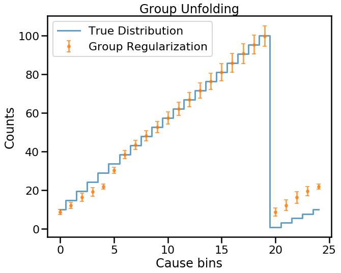
Since the groups are differentiable in terms of response structure and efficiencies, we obtain reasonable unfolding results even using the default uniform prior across all bins!

This simply illustrates the need for proper understanding of one’s data.