Note

This page was generated from docs/source/notebooks/regularization.ipynb. An interactive version of this notebook can be run using Binder by clicking

Note that if you wish to run this notebook on your own, you’ll need to have matplotlib and seaborn installed.

Smoothing unfolded distributions via spline regularization

from pyunfold import iterative_unfold
from pyunfold.callbacks import Logger

import numpy as np
np.random.seed(2)
import matplotlib.pyplot as plt
import seaborn as sns

%matplotlib inline

sns.set_context(context='poster')
plt.rcParams['figure.figsize'] = (10, 8)
plt.rcParams['lines.markeredgewidth'] = 2

Example dataset

We’ll generate the same example dataset that is used in the Getting Started tutorial, i.e. a Gaussian sample that is smeared by some noise.

# True distribution
num_samples = int(1e5)
true_samples = np.random.normal(loc=10.0, scale=4.0, size=num_samples)
bins = np.linspace(0, 20, 21)
num_causes = len(bins) - 1
data_true, _ = np.histogram(true_samples, bins=bins)

# Observed distribution
random_noise = np.random.normal(loc=0.3, scale=0.5, size=num_samples)
observed_samples = true_samples + random_noise
data_observed, _ = np.histogram(observed_samples, bins=bins)
data_observed_err = np.sqrt(data_observed)

# Efficiencies
efficiencies = np.ones_like(data_observed, dtype=float)
efficiencies_err = np.full_like(efficiencies, 0.1, dtype=float)

# Response matrix
response_hist, _, _ = np.histogram2d(observed_samples, true_samples, bins=bins)
response_hist_err = np.sqrt(response_hist)

# Normalized response
column_sums = response_hist.sum(axis=0)
normalization_factor = efficiencies / column_sums

response = response_hist * normalization_factor
response_err = response_hist_err * normalization_factor

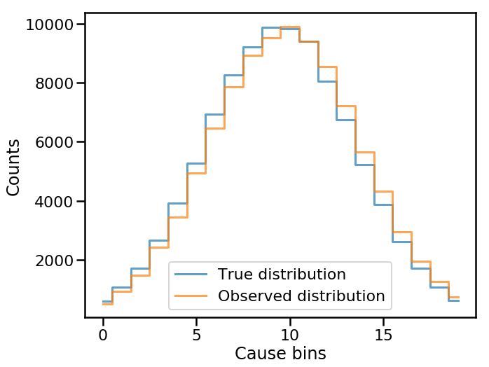
We can see what the true and observed distributions look like for this example dataset

fig, ax = plt.subplots()
ax.step(np.arange(num_causes), data_true, where='mid', lw=3,
        alpha=0.7, label='True distribution')
ax.step(np.arange(num_causes), data_observed, where='mid', lw=3,
        alpha=0.7, label='Observed distribution')
ax.set(xlabel='Cause bins', ylabel='Counts')
ax.legend()
plt.show()

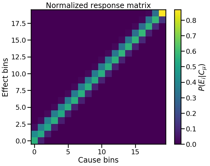
as well as the normalized response matrix

fig, ax = plt.subplots()
im = ax.imshow(response, origin='lower')
cbar = plt.colorbar(im, label='$P(E_i|C_{\mu})$')
ax.set(xlabel='Cause bins', ylabel='Effect bins',
       title='Normalized response matrix')
plt.show()

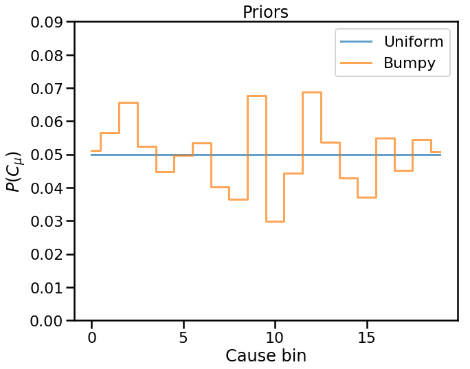
Non-smooth prior

In many experimental setups, we expect the true cause distribution to be fairly smooth. What if we try some bumpy, potentially non-smooth prior?

from pyunfold.priors import uniform_prior

# Uniform prior
uni_prior = uniform_prior(num_causes)

# Random bumpy prior
bumpy_prior = np.abs(np.random.normal(loc=1, scale=0.23, size=num_causes))
bumpy_prior = bumpy_prior / bumpy_prior.sum()

fig, ax = plt.subplots()
plt.step(np.arange(num_causes), uni_prior, where='mid', lw=3,
         alpha=0.7, label='Uniform')
plt.step(np.arange(num_causes), bumpy_prior, where='mid', lw=3,
         alpha=0.7, label='Bumpy')

plt.title('Priors')
plt.xlabel('Cause bin')
plt.ylabel('$P(C_{\mu})$')
plt.ylim(0, 0.09)
plt.legend()
plt.show()

print("Running with bumpy prior...")
unfolded_results_bumpy = iterative_unfold(data=data_observed,
                                          data_err=data_observed_err,
                                          response=response,
                                          response_err=response_err,
                                          efficiencies=efficiencies,
                                          efficiencies_err=efficiencies_err,
                                          prior=bumpy_prior,
                                          ts='ks',
                                          ts_stopping=0.01,
                                          callbacks=[Logger()])

print('\nRunning with uniform prior...')
unfolded_uniform = iterative_unfold(data=data_observed,
                                    data_err=data_observed_err,
                                    response=response,
                                    response_err=response_err,
                                    efficiencies=efficiencies,
                                    efficiencies_err=efficiencies_err,
                                    ts='ks',
                                    ts_stopping=0.01,
                                    callbacks=[Logger()])

Running with bumpy prior...
Iteration 1: ts = 0.1642, ts_stopping = 0.01
Iteration 2: ts = 0.0099, ts_stopping = 0.01

Running with uniform prior...
Iteration 1: ts = 0.1460, ts_stopping = 0.01
Iteration 2: ts = 0.0060, ts_stopping = 0.01

fig, ax = plt.subplots()
plt.step(np.arange(num_causes), data_true, where='mid', lw=3,
         alpha=0.7,
         label='True distribution')

plt.errorbar(np.arange(num_causes), unfolded_uniform['unfolded'],
             yerr=unfolded_uniform['sys_err'],
             alpha=0.7,
             elinewidth=3,
             capsize=4,
             ls='None', marker='.', ms=10,
             label='Unfolded - Uniform Prior')

plt.errorbar(np.arange(num_causes), unfolded_results_bumpy['unfolded'],
             yerr=unfolded_results_bumpy['sys_err'],
             alpha=0.7,
             elinewidth=3,
             capsize=4,
             ls='None', marker='.', ms=10,
             label='Unfolded - Bumpy Prior')

plt.xlabel('Cause bins')
plt.ylabel('Counts')
plt.legend(loc='best', frameon=True)
plt.show()

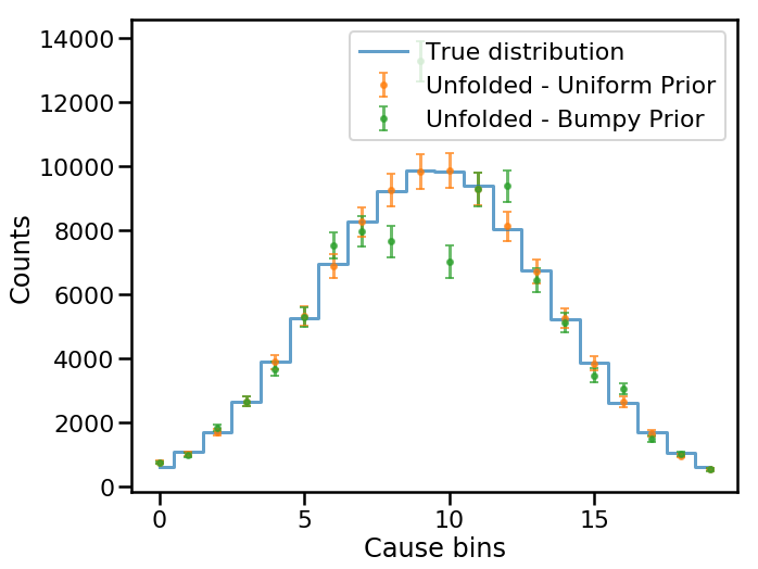
Clearly, the non-smooth initial prior has a strong influence on the unfolded spectrum. This is one potential pitfall: the initial prior informs the procedure as to what properties we think the true distribution has. Unlike for the uniform case, the bumpy prior tells the unfolding algorithm that the true distribution may be bumpy, so the results are also bumpy.

Regularization

We can try to ameliorate this bumpiness by smoothing or regularizing during the unfolding procedure. Here, we can tune the univariate SplineRegularizer routine accessible from the pyunfold.callbacks module.

from pyunfold.callbacks import SplineRegularizer

spline_reg = SplineRegularizer(degree=2, smooth=5e6)

unfolded_results_bumpy_reg = iterative_unfold(data=data_observed,
                                              data_err=data_observed_err,
                                              response=response,
                                              response_err=response_err,
                                              efficiencies=efficiencies,
                                              efficiencies_err=efficiencies_err,
                                              prior=bumpy_prior,
                                              ts='ks',
                                              ts_stopping=0.01,
                                              callbacks=[Logger(), spline_reg])

Iteration 1: ts = 0.1634, ts_stopping = 0.01
Iteration 2: ts = 0.0133, ts_stopping = 0.01
Iteration 3: ts = 0.0143, ts_stopping = 0.01
Iteration 4: ts = 0.0060, ts_stopping = 0.01

fig, ax = plt.subplots()
plt.step(np.arange(num_causes), data_true, where='mid', lw=3,
         alpha=0.7,
         label='True distribution')

plt.errorbar(np.arange(num_causes), unfolded_results_bumpy['unfolded'],
             yerr=unfolded_results_bumpy['sys_err'],
             alpha=0.7,
             elinewidth=3,
             capsize=4,
             ls='None', marker='.', ms=10,
             label='No Regularization')

plt.errorbar(np.arange(num_causes), unfolded_results_bumpy_reg['unfolded'],
             yerr=unfolded_results_bumpy_reg['sys_err'],
             alpha=0.7,
             elinewidth=3,
             capsize=4,
             ls='None', marker='.', ms=10,
             label='With Regularization')

plt.title('Bumpy Initial Priors')
plt.xlabel('Cause bins')
plt.ylabel('Counts')
plt.legend(loc='best', frameon=True)
plt.show()

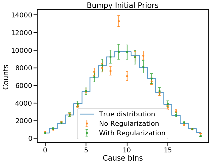
The regularized unfolded result is indeed more consistent with the true distribution, but at the cost of taking a couple of extra iterations to converge, and thus has slightly larger uncertainties due to more mixing.

For this example, a strong regularization parameter (smooth = 5e6) was needed to return consistent unfolded results. Assuming a smooth initial prior is the proper way to avoid this potential issue, unless one does indeed have overriding assumptions regarding smoothness.