GitHub repo with materials:
https://github.com/jrbourbeau/madpy-ml-sklearn-2018
Slides:
https://jrbourbeau.github.io/madpy-ml-sklearn-2018
Contact:
E-mail: james@jamesbourbeau.com
GitHub: jrbourbeau
LinkedIn: jrbourbeau
Source code for plotting Python module can be found on GitHub with the rest of the materials for this talk
import plotting
import numpy as np
np.random.seed(2)
%matplotlib inline
Supervised machine learning workflow

Image source: Model evaluation, model selection, and algorithm selection in machine learning by Sebastian Raschka
Outline
What is machine learning?
Classical programming vs. machine learning
Supervised machine learning
scikit-learn:
Data representation
Estimator API
Example algorithm: decision tree classifier
Model validation
Cross validation
Validation curves
Machine learning vs. classical programming
Classical programming
Devise a set of rules (an algorithm) that are used to accomplish a task
For example, labeling e-mails as either "spam" or "not spam"
def spam_filter(email):
    """Function that labels an email as 'spam' or 'not spam'
    """
    if 'Act now!' in email.contents:
        label = 'spam'
    elif 'hotmail.com' in email.sender:
        label = 'spam'
    elif email.contents.count('$') > 20:
        label = 'spam'
    else:
        label = 'not spam'

    return label
Machine learning
"Field of study that gives computers the ability to learn without being explicitly programmed" — Arthur Samuel (1959)
"A machine-learning system is trained rather than explicitly programmed. It’s presented with many examples relevant to a task, and it finds statistical structure in these examples that eventually allows the system to come up with rules for automating the task." — Francois Chollet, Deep Learning with Python
Supervised machine learning
From a labeled dataset, an algorithm learns a mapping between input data and the desired output label
Goal is to have model generalize well to future, yet unseen, data
Supervised machine learning is further divided into two types of problems:
Classification — Labels are discrete. E.g. determine if a picture is of a cat, dog, or person.
Regression — Labels are continuous. E.g. predict home prices.
plotting.plot_classification_vs_regression()

Machine learning in Python with scikit-learn
scikit-learn
Popular Python machine learning library
Designed to be a well documented and approachable for non-specialist
Built on top of NumPy and SciPy
scikit-learn can be easily installed with
piporcondapip install scikit-learnconda install scikit-learn
API design for machine learning software: experiences from the scikit-learn project — for a discusses of the API design choices for scikit-learn
Data representation in scikit-learn
Training dataset is described by a pair of matrices, one for the input data and one for the output
Most commonly used data formats are a NumPy
ndarrayor a PandasDataFrame/Series
Each row of these matrices corresponds to one sample of the dataset
Each column represents a quantitative piece of information that is used to describe each sample (called "features")
plotting.plot_data_representation()

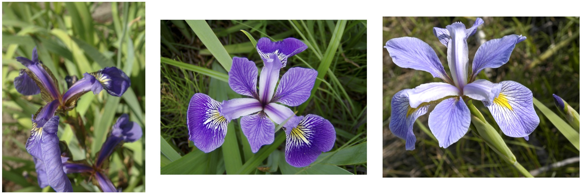
Iris dataset
Dataset consists of 150 samples (individual flowers) that have 4 features: sepal length, sepal width, petal length, and petal width (all in cm)
Each sample is labeled by its species: Iris Setosa, Iris Versicolour, Iris Virginica
Task is to develop a model that predicts iris species
Iris dataset is freely available from the UCI Machine Learning Repository
Loading the iris dataset from scikit-learn
from sklearn.datasets import load_iris

X, y = load_iris(return_X_y=True)
# Only include first two training features (sepal length and sepal width)
X = X[:, :2]

print(f'First 5 samples in X: \n{X[:5]}')
print(f'Labels: \n{y}')
plotting.plot_2D_iris()

Estimators in scikit-learn
Algorithms are implemented as estimator classes in scikit-learn
Each estimator in scikit-learn is extensively documented (e.g. the KNeighborsClassifier documentation) with API documentation, user guides, and example usages.
from sklearn.tree import DecisionTreeClassifier, DecisionTreeRegressor
from sklearn.neighbors import KNeighborsClassifier, KNeighborsRegressor
from sklearn.ensemble import RandomForestClassifier, GradientBoostingRegressor
from sklearn.svm import SVC, SVR
from sklearn.linear_model import LinearRegression, LogisticRegression
- A model is an instance of one of these estimator classes
model = KNeighborsClassifier(n_neighbors=5)
print(model)
Estimator API
class Estimator(BaseClass):

    def __init__(self, **hyperparameters):
        # Setup Estimator here

    def fit(self, X, y):
        # Implement algorithm here

        return self

    def predict(self, X):
        # Get predicted target from trained model
        # Note: fit must be called before predict

        return y_pred
Training a model — fit then predict
# Create the model
model = KNeighborsClassifier(n_neighbors=5)

# Fit the model
model.fit(X, y)

# Get model predictions
y_pred = model.predict(X)
y_pred
Example algorithm: decision tree classifier
Decision tree classifier
Idea behind the decision tree algorithm is to sequentially partition a training dataset by asking a series of questions.

Image source: Raschka, Sebastian, and Vahid Mirjalili. Python Machine Learning, 2nd Ed. Packt Publishing, 2017.
Node splitting to maximize purity

Decision tree classifier in scikit-learn
from sklearn.tree import DecisionTreeClassifier

clf = DecisionTreeClassifier(max_depth=2)
clf.fit(X, y)
Visualizing decision trees — tree graph
plotting.plot_decision_tree(clf)
Visualizing decision trees — decision regions
plotting.plot_tree_decision_regions(clf)

Model validation
Model performance metrics
There are many different performance metrics for classification and regression problems. Which metric you should use depends on the particular problem you are working on
Many commonly used performance metrics are built into the
metricssubpackage in scikit-learnHowever, a user-defined scoring function can be created using the
sklearn.metrics.make_scorerfunction
# Classification metrics
from sklearn.metrics import (accuracy_score, precision_score,
                             recall_score, f1_score, log_loss)
# Regression metrics
from sklearn.metrics import mean_squared_error, mean_absolute_error, r2_score
y_pred = [0, 2, 1, 3, 1]
y_true = [0, 1, 1, 3, 2]
accuracy_score(y_true, y_pred)
mean_squared_error(y_true, y_pred)
Separate training & testing sets
A trained model will generally perform better on data that was used to train it
Want to measure how well a model generalizes to new, unseen data
Need to have two separate datasets. One for training models and one for evaluating model performance
scikit-learn has a convenient
train_test_splitfunction that randomly splits a dataset into a testing and training set
from sklearn.model_selection import train_test_split

X_train, X_test, y_train, y_test = train_test_split(X, y, test_size=0.2,
                                                    random_state=2)

print(f'X.shape = {X.shape}')
print(f'X_test.shape = {X_test.shape}')
print(f'X_train.shape = {X_train.shape}')
clf = DecisionTreeClassifier()
clf.fit(X_train, y_train)
print(f'training accuracy = {accuracy_score(y_train, clf.predict(X_train))}')
print(f'testing accuracy = {accuracy_score(y_test, clf.predict(X_test))}')
Model selection — hyperparameter optimization
Choose model hyperparameter values to avoid under- and over-fitting
Under-fitting — model isn't sufficiently complex enough to properly model the dataset at hand
Over-fitting — model is too complex and begins to learn the noise in the training dataset

Image source: Underfitting vs. Overfitting in scikit-learn examples
$k$-fold cross validation diagram

Image source: Raschka, Sebastian, and Vahid Mirjalili. Python Machine Learning, 2nd Ed. Packt Publishing, 2017.
Cross validation in scikit-learn
from sklearn.model_selection import cross_validate

clf = DecisionTreeClassifier(max_depth=2)
scores = cross_validate(clf, X_train, y_train,
                        scoring='accuracy', cv=10,
                        return_train_score=True)

print(scores.keys())
test_scores = scores['test_score']
train_scores = scores['train_score']
print(test_scores)
print(train_scores)

print('\n10-fold CV scores:')
print(f'training score = {np.mean(train_scores)} +/- {np.std(train_scores)}')
print(f'validation score = {np.mean(test_scores)} +/- {np.std(test_scores)}')
Validation curves
Validation curves are a good way to diagnose if a model is under- or over-fitting
plotting.plot_validation_curve()

plotting.plot_max_depth_validation(clf, X_train, y_train)

Hyperparameter tuning via GridSearchCV
In practice, you'll want to optimize many different hyperparameter values simultaneously
The
GridSearchCVobject in scikit-learn'smodel_selectionsubpackage can be used to scan over many different hyperparameter combinationsCalculates cross-validated training and testing scores for each hyperparameter combinations
The combination that maximizes the testing score is deemed to be the "best estimator"
from sklearn.model_selection import GridSearchCV

# Instantiate a model
clf = DecisionTreeClassifier()

# Specify hyperparameter values to test
parameters = {'max_depth': range(1, 20),
              'criterion': ['gini', 'entropy']}

# Run grid search
gridsearch = GridSearchCV(clf, parameters, scoring='accuracy', cv=10)
gridsearch.fit(X_train, y_train)

# Get best model
print(f'gridsearch.best_params_ = {gridsearch.best_params_}')
print(gridsearch.best_estimator_)
Supervised machine learning workflow
Image source: Model evaluation, model selection, and algorithm selection in machine learning by Sebastian Raschka
Step 1 — Separate training and testing datasets

Image source: Model evaluation, model selection, and algorithm selection in machine learning by Sebastian Raschka
X_train, X_test, y_train, y_test = train_test_split(X, y, test_size=0.3,
                                                    random_state=2)
Steps 2 & 3 — Optimize hyperparameters via cross validation

Image source: Model evaluation, model selection, and algorithm selection in machine learning by Sebastian Raschka
clf = DecisionTreeClassifier()
parameters = {'max_depth': range(1, 20),
              'criterion': ['gini', 'entropy']}
gridsearch = GridSearchCV(clf, parameters, scoring='accuracy', cv=10)
gridsearch.fit(X_train, y_train)
print(f'gridsearch.best_params_ = {gridsearch.best_params_}')

best_clf = gridsearch.best_estimator_
best_clf
Steps 4 — Model performance

Image source: Model evaluation, model selection, and algorithm selection in machine learning by Sebastian Raschka
y_pred = best_clf.predict(X_test)
test_acc = accuracy_score(y_test, y_pred)
print(f'test_acc = {test_acc}')
Steps 5 — Train final model on full dataset

Image source: Model evaluation, model selection, and algorithm selection in machine learning by Sebastian Raschka
final_model = DecisionTreeClassifier(**gridsearch.best_params_)
final_model.fit(X, y)
Iris classification problem
# Step 1: Get training and testing datasets
X_train, X_test, y_train, y_test = train_test_split(X, y, test_size=0.3,
                                                    random_state=2)

# Step 2: Use GridSearchCV to find optimal hyperparameter values
clf = DecisionTreeClassifier(random_state=2)
parameters = {'max_depth': range(1, 20),
              'criterion': ['gini', 'entropy']}
gridsearch = GridSearchCV(clf, parameters, scoring='accuracy', cv=10)
gridsearch.fit(X_train, y_train)
print(f'gridsearch.best_params_ = {gridsearch.best_params_}')

# Step 3: Get model with best hyperparameters
best_clf = gridsearch.best_estimator_

# Step 4: Get best model performance from testing set
y_pred = best_clf.predict(X_test)
test_acc = accuracy_score(y_test, y_pred)
print(f'test_acc = {test_acc}')

# Step 5: Train final model on full dataset
final_model = DecisionTreeClassifier(random_state=2, **gridsearch.best_params_)
final_model.fit(X, y);